Homogeneous Coordinates and Projective Geometry
If you work in computer graphics, you deal with the following operations every day:
- A point in 3D space is written as a 4D vector $(x,y,z,w)$.
- $(x,y,z,w)$ and $(kx,ky,kz,kw)\;(k \neq 0)$ represent the same point.
- At render time, you perform a “perspective divide”: $(x/w,\;y/w,\;z/w)$.
- $w=0$ is treated as a “direction”—a point at infinity.
This design is not a graphics programmer’s invention. Its roots lie in 19th-century projective geometry. Homogeneous coordinates are not an engineering hack; they are the most natural coordinate system for projective space.
Where Projective Geometry Comes From
Any two lines intersect—this is the core conviction of projective geometry.
In Euclidean geometry, this is clearly false: parallel lines never meet. But stand between railroad tracks and look into the distance—the two rails do “meet” on the horizon. Renaissance painters figured this out long ago; the development of perspective forced an inescapable question:
How do you describe, in algebraic language, the intersection of two lines—whether that intersection is at a finite point or at infinity?
The answer is simple: introduce points at infinity.
The basic setup: in ordinary affine space (i.e., $\mathbb{R}^n$), attach a “point at infinity” to every direction. Then a family of parallel lines all meet at the same point at infinity. The space obtained after adding these new points is called projective space.
A Geometric Feel for the Projective Plane
Before diving into algebra, let’s build some geometric intuition.
Imagine standing on a long straight road looking ahead. The road edges, guardrails, rows of trees—all these originally parallel lines converge to a single point in the distance. That is the vanishing point. Turn your head in another direction, and another family of parallel lines converges to a different vanishing point. All vanishing points for lines parallel to the ground lie on the horizon.
That “horizon line” is, in projective geometry, the line at infinity—and it is no different in nature from any ordinary line you draw on paper. As you turn, the vanishing point slides along the horizon, but the horizon remains the horizon. What projective geometry does is abstract this visually intuitive geometric structure into an axiom system with no “parallel exception.”
Even more interesting are the conic sections. In Euclidean plane geometry, ellipses, parabolas, and hyperbolas are classified as three completely different things. But in the projective plane, they are a single kind of object—a non-degenerate conic:
| Curve type | Relationship to the line at infinity |
|---|---|
| Ellipse | No intersection (stays entirely in the finite region) |
| Parabola | Tangent (escapes to infinity along the opening direction) |
| Hyperbola | Intersects at two points (the two branches approach different directions at infinity) |
Once you treat the line at infinity as an ordinary line, the difference among the three curves reduces to simply “0 intersections, 1 tangency, 2 intersections”—no more fundamental than asking how many times an ordinary line intersects a circle. This is the beauty of projective geometry: infinity is leveled.
As an aside, the projective plane has an extraordinarily elegant property—duality. In Euclidean geometry, “two points determine a line” is always true, but “two lines determine a point” has an annoying exception—parallel lines do not intersect. In projective geometry, that exception disappears: any two lines intersect. Thus “two points determine a line” and “two lines determine a point” become perfectly symmetric propositions. This means every theorem in projective geometry automatically yields a dual theorem by swapping “point” and “line”—no need to prove it again.
Now the question is: how do you represent these newly added points at infinity with coordinates?
Algebraic Construction of Projective Space
We need a coordinate system that expresses finite points and points at infinity in a unified form.
The Construction Idea
Consider all lines through the origin in $\mathbb{R}^{n+1}$. Intuitively:
- Every line through the origin has a unique intersection with the affine hyperplane $x\_0 = 1$ (provided the line is not parallel to that hyperplane). This intersection is a “finite point.”
- If the line happens to be parallel to $x\_0 = 1$ (i.e., $x\_0 = 0$), it has no intersection with the hyperplane—but it gives a “direction,” corresponding exactly to a point at infinity.
Formal Definition
On $\mathbb{R}^{n+1} \setminus \lbrace \mathbf{0}\rbrace$, define the equivalence relation $\sim$:
That is, two non-zero vectors are equivalent if and only if they lie on the same line through the origin.
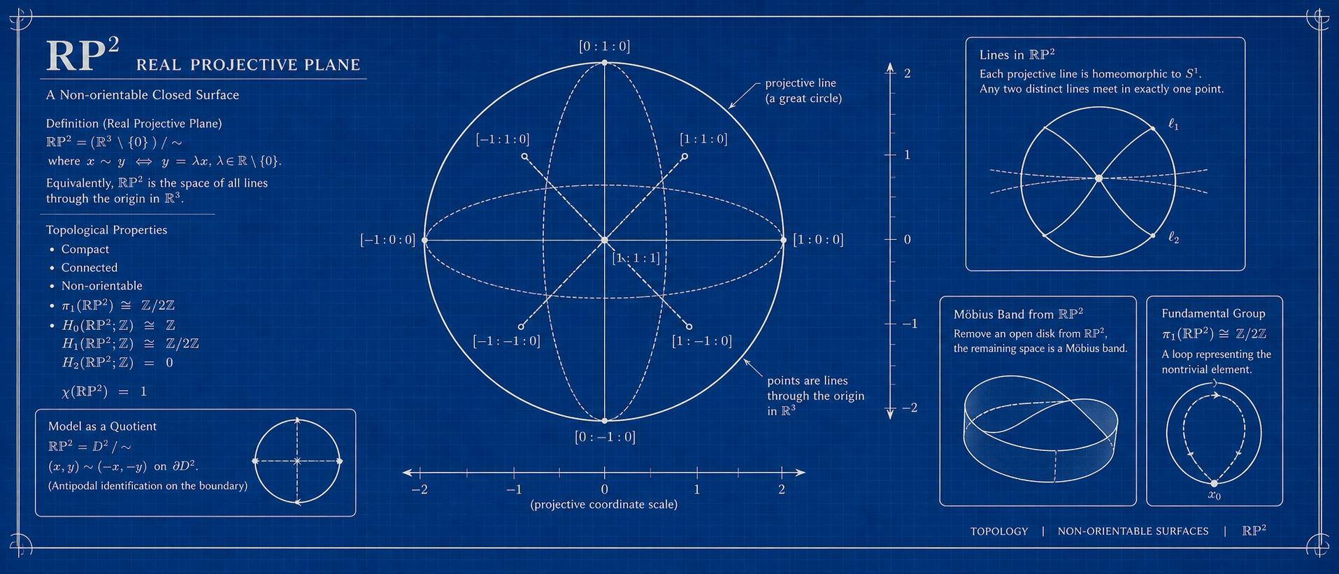
Define $n$-dimensional real projective space:
Each element of $\mathbb{RP}^n$ is an equivalence class of lines through the origin. Denote the equivalence class by:
This tuple $[x\_0 : x\_1 : \cdots : x\_n]$ is called the homogeneous coordinates of the projective point. By the definition of the equivalence relation:
That is—homogeneous coordinates are unique only up to a non-zero scalar multiple. This is precisely the mathematical origin of the graphics rule “$(x,y,z,w)$ and $(kx,ky,kz,kw)$ represent the same point.”
The origin is excluded from $\mathbb{RP}^n$ so that equivalence classes are well-defined (the origin itself is a degenerate case, not equivalent to any non-zero vector). The equivalence relation satisfies reflexivity, symmetry, and transitivity—verification is straightforward.
How Homogeneous Coordinates Unify Finite and Infinite
Now let’s see how homogeneous coordinates in $\mathbb{RP}^n$ accommodate both finite points and points at infinity.
Affine Charts
Take the points in $\mathbb{RP}^n$ with $x\_0 \neq 0$. Normalize the homogeneous coordinates:
This yields ordinary coordinates in $\mathbb{R}^n$:
This is the familiar affine coordinate. The map
is an embedding, placing $\mathbb{R}^n$ as a dense open subset of $\mathbb{RP}^n$.
Points at Infinity
When $x\_0 = 0$, the homogeneous coordinates take the form:
These cannot be normalized to $[1 : \cdots]$—they are points at infinity. This tuple of coordinates describes a direction: the direction of the vector $(x\_1,\ldots,x\_n)$.
The set of all points at infinity is precisely $\mathbb{RP}^{n-1}$ (a projective space of one dimension lower). This gives the classical decomposition of $\mathbb{RP}^n$ into an affine part and a part at infinity:
$\mathbb{R}^n$ is the affine chart; $\mathbb{RP}^{n-1}$ is the hyperplane at infinity.
In graphics, $(x,y,z,0)$ represents a direction vector rather than a position—the mathematical essence lies right here.
Points at Infinity: One or Infinitely Many?
Beginners are often confused: is the point at infinity added to $\mathbb{R}^n$ a single point, or infinitely many? Both claims seem to appear in different contexts.
The answer is—both are correct, depending on which compactification you use.
Consider first the one-point compactification (also called Alexandroff compactification). Add one point $\infty$ to $\mathbb{R}^n$, with neighborhoods of $\infty$ defined as complements of compact sets. The resulting space is homeomorphic to $S^n$ (the $n$-dimensional sphere). For $n=2$, the Riemann sphere $S^2$ from complex analysis is precisely the one-point compactification of the complex plane $\mathbb{C} \cong \mathbb{R}^2$. In this model, “infinity” in all directions is glued into a single point.
Now consider the projective construction. In $\mathbb{RP}^n = (\mathbb{R}^{n+1}\setminus\lbrace \mathbf{0}\rbrace)/\sim$, the set of all points at infinity consists of equivalence classes with $x\_0 = 0$, which form exactly $\mathbb{RP}^{n-1}$. For $n=2$, $\mathbb{RP}^1$ is homeomorphic to $S^1$—the points at infinity form a circle, with uncountably many points.
The key distinction: projective geometry requires infinitely many points at infinity. Because—
Families of parallel lines in different directions meet at different points at infinity. If there were only one point at infinity, lines in all directions would intersect at the same point, collapsing the entire geometric structure. The richness of projective geometry (e.g., the projective classification of quadrics) exists precisely because each direction gets its own independent point at infinity.
Summary: One-point compactification ($S^n$) has exactly 1 point at infinity; projective compactification ($\mathbb{RP}^n$) has infinitely many, forming $\mathbb{RP}^{n-1}$. The homogeneous coordinate system in graphics corresponds to the latter—the $(x,y,z)$ in $(x,y,z,0)$ is there to distinguish different directions. The sole exception is $n=1$: $\mathbb{RP}^0$ is a single point, so the two compactifications coincide ($S^1 \cong \mathbb{RP}^1$).
The Essence of Perspective Division
In the graphics pipeline, the vertex shader outputs 4D homogeneous coordinates $(x,y,z,w)$, after which the GPU automatically performs the perspective divide:
This is precisely the operation of normalizing homogeneous coordinates onto the affine chart $w=1$. $w$ is exactly the $x\_0$ from the construction above. It is that simple.
Projective Transformations
With projective space $\mathbb{RP}^n$ in hand, we can discuss transformations on it.
Definition
A projective transformation on $\mathbb{RP}^n$ is induced by an invertible $(n+1) \times (n+1)$ real matrix $M \in GL(n+1,\mathbb{R})$:
$\mathbf{x}$ and $\mathbf{y}$ are homogeneous coordinate vectors (column vectors). Note:
- Since homogeneous coordinates are defined only up to a scalar multiple, $M$ and $\lambda M\;(\lambda \neq 0)$ represent the same projective transformation.
- Hence the projective transformation group is isomorphic to $PGL(n+1,\mathbb{R}) := GL(n+1,\mathbb{R}) / \mathbb{R}^\times$.
Let’s use the most common case in graphics, $n=3$, to derive why the degrees of freedom are $15$.
Consider a $4 \times 4$ real matrix:
At first glance there are $4 \times 4 = 16$ parameters. But in the projective transformation $\mathbf{y} = M\mathbf{x}$, homogeneous coordinates themselves are projectively equivalent: $[x\_0:x\_1:x\_2:x\_3] = [\lambda x\_0:\lambda x\_1:\lambda x\_2:\lambda x\_3]$. This means multiplying the entire matrix $M$ by an arbitrary non-zero scalar $\lambda$:
induces the exact same transformation. Because $(\lambda M)\mathbf{x} = \lambda(M\mathbf{x})$, and $\lambda(M\mathbf{x})$ and $M\mathbf{x}$ represent the same projective point (homogeneous coordinates differ by a scalar multiple).
Thus 1 of those 16 parameters is redundant—the overall scalar factor produces no new transformation. The number of independent parameters:
An equivalent perspective: since the overall scalar does not affect the transformation, you can fix one non-zero matrix entry to $1$ (as long as it was not originally $0$), turning 16 parameters into 15. For instance, if $m\_{00} \neq 0$, normalize to $m\_{00}=1$, leaving 15 free parameters. This is why a $4 \times 4$ projection matrix in graphics typically has 15 (rather than 16) independently adjustable components.
In general, for $\mathbb{RP}^n$, the projective transformation group is $PGL(n+1,\mathbb{R})$, with $(n+1)^2 - 1$ degrees of freedom.
What Projective Transformations Preserve
Projective transformations preserve two fundamental geometric quantities: collinearity and the cross-ratio.
- If three points are collinear, their images under a projective transformation remain collinear.
- If $A,B,C,D$ are four points on a line, the cross-ratio is invariant under projective transformations.
Conversely, any bijection that preserves collinearity must be a projective transformation—this is a fundamental theorem of projective geometry (von Staudt).
Affine Transformations as a Subgroup
Everyone in graphics knows that the Model and View matrices are both $4 \times 4$—and they share a common structural feature. This is no coincidence.
Matrix Form of Affine Transformations
An affine transformation on $\mathbb{R}^n$ takes the form $\mathbf{y} = A\mathbf{x} + \mathbf{t}$, with $A \in GL(n,\mathbb{R})$, $\mathbf{t} \in \mathbb{R}^n$.
In homogeneous coordinates (using the $[x\_0 : x\_1 : \cdots : x\_n]$ notation, with $x\_0$ as the homogeneous component), this affine transformation is written as an $(n+1) \times (n+1)$ matrix:
Verification: for a point $[1:\mathbf{x}]$ on the affine chart, i.e., the column vector $[1,\;\mathbf{x}^T]^T$:
After normalization this yields exactly $A\mathbf{x} + \mathbf{t}$. ($\mathbf{x},\mathbf{t}$ are both column vectors.)
Why Affine Transformations Preserve $x\_0$
Observe the effect of an affine transformation on a point at infinity $[0:\mathbf{v}]$ (column vector $[0,\;\mathbf{v}^T]^T$):
The result is still a point at infinity ($x\_0 = 0$). In other words, affine transformations map points at infinity to points at infinity—they do not send finite points to infinity, nor vice versa. This matches our real-world intuition: translation and rotation do not “push” ordinary objects off to infinity.
Conversely, if the first row of the matrix is not $[1\;0\;\cdots\;0]$, finite points can be mapped to $x\_0=0$ (infinity), and vice versa. Such transformations are non-affine projective transformations—perspective projection is precisely of this kind.
Notation note: In graphics, homogeneous coordinates usually place $w$ at the end: $(x,y,z,w)$. In that convention, the affine matrix is written as $\begin{bmatrix} A & \mathbf{t} \\ \mathbf{0}^T & 1 \end{bmatrix}$ (last row $[0\;0\;0\;1]$). The two conventions are essentially the same, differing only in the ordering of coordinates. The mathematical sections of this article use the $x\_0$-first convention.
Degrees of Freedom
In the affine transformation, $A$ contributes $n^2$ degrees of freedom, $\mathbf{t}$ contributes $n$, summing to $n^2 + n$. For $n=3$ this is $12$, which is $3$ fewer than the $15$ of a general projective transformation—those missing $3$ degrees of freedom come exactly from the three positions in the first row $\mathbf{0}^T$ (they must be zero to preserve $x\_0$).
Perspective Projection: A Graphics Example
This section is the most “engineering” part of this article. We examine how the standard perspective projection matrix fits naturally into the projective transformation framework.
Notation convention: This section uses the graphics convention—homogeneous coordinates written as $(x,y,z,w)$, with $w$ at the end. The matrix form is adjusted accordingly (affine transform with last row $[0\;0\;0\;1]$). This is essentially the same as the $x\_0$-first convention used in the earlier mathematical sections.
Problem Setup
Given a symmetric view frustum:
- Near clip plane distance (along the $-z$ direction): $n > 0$
- Far clip plane distance: $f > n$
- On the near clip plane, $x$ range $[-r, r]$, $y$ range $[-t, t]$
Goal: map this frustum into the NDC cube $[-1,1]^3$.
Deriving the Projection Matrix
In eye space, the viewpoint is at the origin, looking down the $-z$ direction. The fundamental relationship of perspective projection:
($z\_e < 0$, so the signs of $x\_p, y\_p$ match those of $x\_e, y\_e$.)
Linearly map $x\_p$ from $[-r, r]$ to $[-1, 1]$:
Similarly:
For depth $z$, we need to map $[-n, -f]$ to $[-1, 1]$. Assume the transformation form:
Plug in the two endpoints:
- $z\_e = -n \implies z\_{ndc} = -1$: $-An + B = n$
- $z\_e = -f \implies z\_{ndc} = 1$: $-Af + B = -f$
Solve this linear system:
Thus:
Writing in Homogeneous Coordinates
In homogeneous coordinates, express all the above operations in matrix form:
Compute $w\_c$:
It equals the negation of the depth in eye space ($z\_e < 0$, so $w\_c > 0$). Note that $w\_c \neq 1$—this is emphatically not an affine transformation.
The subsequent perspective divide:
is exactly the normalization of homogeneous coordinates onto the $w=1$ affine chart.
Key Observations
The last row of the projection matrix is $[0\;0\;-1\;0]$, not $[0\;0\;0\;1]$. This means:
- This is a genuine projective transformation, not an affine one. It maps finite points into a state that requires perspective division to recover.
- The essence of perspective division is homogeneous coordinate normalization. Dividing by $w$ is picking an affine chart representative.
- The farther the object ($|z\_e|$ larger), the larger $w\_c$ is, and the smaller the coordinate after perspective division—this is the algebraic root of “closer objects appear larger.”
The last row of the Model and View matrices is always $[0\;0\;0\;1]$; they are affine transformations through and through, and do not alter the $w$ component. This is the essential difference between rotation/translation/scaling and perspective projection.
The Invariant of Projective Transformations: Cross-Ratio
Projective transformations are less rigid than rigid-body transformations (they no longer preserve lengths, angles, or even parallelism), but they still preserve some structure. The most important projective invariant is the cross-ratio.
Definition
Let $A,B,C,D$ be four distinct points on a projective line, with homogeneous coordinate representations $\mathbf{a},\mathbf{b},\mathbf{c},\mathbf{d} \in \mathbb{R}^2$.
The cross-ratio is defined as:
where $\det(\mathbf{x},\mathbf{y}) = x\_1y\_2 - x\_2y\_1$.
On an affine chart, if all four points are affine points, this definition reduces to the more familiar form:
where $AC$ etc. denote signed distances.
Cross-Ratio is a Projective Invariant
Proposition: The cross-ratio is invariant under projective transformations.
Proof: Let the projective transformation be induced by $M \in GL(2,\mathbb{R})$ (the $\mathbb{RP}^1$ case), with $\mathbf{x} \mapsto M\mathbf{x}$. Substitute:
The determinants in both the numerator and denominator pick up the same factor $\det(M)$, which cancels in the ratio. The same reasoning applies in higher dimensions.
The cross-ratio is the most important numerical invariant of projective geometry: the cross-ratios of two 4-tuples of points are equal if and only if there exists a projective transformation mapping one 4-tuple to the other.
$SO(3) \cong \mathbb{RP}^3$: The Topological Nature of Rotation
This section ties together three seemingly unrelated things: quaternion rotations, projective space, and gimbal lock. Their common root is—the topological structure of the 3D rotation group is a projective space.
Honestly, I think this is the coolest part.
Unit Quaternions and $SO(3)$
Denote the quaternion algebra $\mathbb{H} = \lbrace a+bi+cj+dk \mid a,b,c,d \in \mathbb{R}\rbrace$, with multiplication satisfying $i^2=j^2=k^2=ijk=-1$ and the Hamilton relations.
Take the unit quaternions $Sp(1) := \lbrace x \in \mathbb{H} \mid |x| = 1\rbrace$ (where $|a+bi+cj+dk| = \sqrt{a^2+b^2+c^2+d^2}$). Identify the pure imaginary quaternions $Im\mathbb{H} = \lbrace bi+cj+dk\rbrace$ with $\mathbb{R}^3$.
Define the conjugation action:
$x \in Sp(1)$, $y \in Im\mathbb{H}$, with quaternion multiplication on the right. Key facts:
- The image lies in $SO(3)$: $\theta\_x$ preserves the inner product ($|xyx^{-1}| = |x||y||x^{-1}| = |y|$), and the determinant is $+1$ ($Sp(1) \cong S^3$ is connected; the determinant as a continuous map must have a connected image, and $\theta\_1 = I$ has determinant $1$, so the entire image must have determinant $1$).
- Kernel of the homomorphism: $\ker\theta = \lbrace 1, -1\rbrace$ (only $\pm 1$ act trivially).
- Surjectivity: the image of $\theta$ is all of $SO(3)$.
By the first isomorphism theorem for groups:
This is the mathematical origin of the rule “$q$ and $-q$ represent the same rotation.”
From $Sp(1)$ to $\mathbb{RP}^3$
$Sp(1)$ is defined by the condition $a^2+b^2+c^2+d^2=1$, which is exactly the unit sphere $S^3$ in $\mathbb{R}^4$:
Gluing antipodal points $x$ and $-x$ on $S^3$ is precisely the standard construction of $\mathbb{RP}^3$:
This result is extraordinarily beautiful: the set of all 3D rotations is, topologically, a 3-dimensional projective space.
Where Gimbal Lock Comes From
Once you know $SO(3) \cong \mathbb{RP}^3$, many things become clear.
$S^3$ is simply connected ($\pi\_1 = 0$), but $\mathbb{RP}^3$ has fundamental group $\pi\_1(\mathbb{RP}^3) \cong \mathbb{Z}\_2$ (because $S^3 \to \mathbb{RP}^3$ is a double cover). This means $SO(3)$ is not simply connected—intuitively, a loop corresponding to a full $360^\circ$ rotation cannot be continuously shrunk to a point in $SO(3)$.
This is the deep reason behind gimbal lock in Euler angle parameterization. Euler angles are essentially an attempt to force a coordinate chart of $S^1 \times S^1 \times S^1$ onto $\mathbb{RP}^3$, but $\mathbb{RP}^3$ is not the product of three circles at all—it is a compact, boundaryless projective space. Using three angles to cover it inevitably creates singularities in the parameterization at certain places (the “polar regions”). Those singularities are gimbal lock.
Why are quaternions immune to gimbal lock? Because they directly use coordinates on $S^3$ (in fact $\mathbb{RP}^3$) to parameterize rotations, without going through an angle decomposition. The fact that $q$ and $-q$ represent the same rotation is precisely the algebraic mirror of the antipodal gluing in $\mathbb{RP}^3$.
That’s it. For someone working in graphics, understanding to this depth should be enough. The rest—differential geometry and Lie groups—we’ll leave aside.