Continuity/Compactness/Connectedness

The Definition of Continuity

In mathematical analysis, we define continuity of a function like this: $f$ is continuous at $x\_0$ if for every $\epsilon$, there exists a $\delta$ such that for every $x \in R^n$, if $\vert \vert x - x\_0 \vert \vert < \delta$, then $\vert \vert f(x) - f(x\_0) \vert \vert < \epsilon$.

And we define an open set in $R^n$ as follows: $U \subset R^n$ is called an open set in $R^n$ if for every $x \in U$, there exists a $\delta$ such that $B(x;\delta) \subset U$, where $B(x;\delta)$ is an open ball.

The relationship between continuity and open sets: if $f:R^n \rightarrow R^m$, then the preimage of every open set under $f$ is open.

Necessity: Consider $f^{-1}(U)$. For any $x\_0 \in f^{-1}(U)$, we have $f(x\_0) \in U$. Since $U$ is open, there exists an $\epsilon$ such that $B(f(x\_0); \epsilon) \subset U$. Since $f$ is continuous at $x\_0$, there exists $\delta > 0$ such that

Therefore

So by the definition of an open set, $f^{-1}(U)$ is open in $R^n$.

Sufficiency: For every $x\_0$ and every $\epsilon$, consider $B(f(x\_0);\epsilon$. By assumption, $f^{-1}(B(f(x\_0);\epsilon))$ is open. By the definition of open sets, there exists $\delta$ such that $B(x\_0;\delta) \subset f^{-1}(B(f(x\_0);\epsilon))$. In other words, for every $x\_0$ and every $\epsilon$, we have $f(B(x\_0;\delta)) \subset B(f(x\_0);\epsilon))$. Thus $f$ is continuous at $x\_0$. Since $x\_0$ was arbitrary, $f$ is a continuous function.

This result is extremely important. It means that continuity of a function can be described entirely by what happens to open sets under the map. So “the preimage of every open set is open” can itself be taken as the definition of continuity.

The definition in analysis actually uses the metric on $R^n$. A metric is like the skeleton of a space. Once a metric is fixed, it is less convenient to make topological transformations of the space. So in topology, the definition of continuity uses a more essential description: the preimage of an open set is open. This lets us define continuous functions even when there is no metric.

Remark

1. The finer a topology is, for example the discrete topology, the more flexible that topological space is. The coarser a topology is, for example the trivial topology, the more rigid that topological space is.

For example, let $X$ be a set and give $X$ the discrete topology. Suppose $f$ is a map from $X$ to another topological space. Then no matter what subset of the target we take and pull back, the preimage is open. That is, under the discrete topology, every map has the property that preimages of open sets are open. So every map from $X$ is continuous. This space is very flexible: we can map it however we like.

As another example, let $X$ be a set and give $X$ the trivial topology. Now take a map $f$ from $X$ to another topological space. If $f$ is continuous, then $f(X)$ must also carry the trivial topology. In this situation, there are very few continuous maps from $X$: they have to map from a trivial topology into a trivial topology. So this space is very rigid and cannot do very much.

2. Continuity is described using preimages. Why not use the image of open sets being open?

If a map sends open sets to open sets, it is called an open map. In fact:

An open map need not be continuous. And the inverse of a continuous function is continuous $\Leftrightarrow$ the map is an open map.

The counterexample is a bit hard to construct. There is an example in Counterexamples in Real Analysis.

Some Propositions

Proposition 1: The composition of continuous maps is continuous.

Proposition 2: If $f$ is continuous and $A$ is a subset of the domain $X$, with $A$ given the subspace topology, then the restriction $f\_A$ to $A$ is also continuous.

Proposition 3: The following statements are equivalent:

1. $f: X \rightarrow Y$ is continuous.
2. Let $\beta$ be a basis for the topology on $Y$. For every $U \in \beta$, $f^{-1}(U)$ is open.
3. For every $A \subset X$, $f(\bar{A}) \subset \bar{f(A)}$.
4. For every $B \subset Y$, $\bar{f^{-1}(B)} \subset f^{-1}(\bar{B})$.
5. The preimage of every closed set is closed.

Statement 2 gives a better way to check continuity in practice: we do not need to check that the preimage of every open set is open; it is enough to check this on a basis. For statement 3, this is obvious from the viewpoint of analysis. It is really saying that continuity is equivalent to limits commuting with the function.

Limits in Topological Spaces

Let $X$ be a topological space and let ${x\_n}$ be a sequence. We say that $x$ is a limit of ${x\_n}$ if, for every open set $U \subset X$ with $x \in U$, there exists $N$ such that for all $n > N$, $x\_n \in U$.

If $X$ is taken to be $R^n$, then the definition above agrees with the definition of the limit of a sequence from analysis. For a general topological space, since there is no metric, we have to define limits using open sets.

One thing to notice is that under this definition, limits need not be unique.

For example, take $X=\lbrace 0, 1 \rbrace$ and $\mathscr{F} = \lbrace \lbrace 0 \rbrace, \lbrace 0,1 \rbrace , \varnothing\rbrace$. Look at the sequence $x\_n=0, n = 1, 2, 3, ...$. Then the limit of $x\_n$ is both $0$ and $1$. This is easy to check.

So we need to add one condition to the topological space. A topological space is called a Hausdorff space if for every $x\_1, x\_2 \in X$ with $x\_1 \neq x\_2$, there exist open sets $U\_1, U\_2$ such that $x\_1 \in U\_1, x\_2 \in U\_2$, and $U\_1 \cap U\_2 = \varnothing$.

This additional condition is called the separation axiom, also known as the T2 axiom.

In a Hausdorff space, if a limit exists, then it is unique: $\lim\_{n \to +\infty}(x\_n) = x$.

The proof is exactly the same as the proof of uniqueness of sequence limits in analysis.

Suppose there are two limits $y\_1, y\_2, y\_1 \neq y\_2$. By the definition of a Hausdorff space, we can find two open sets $U\_1,U\_2$ containing $y\_1,y\_2$ respectively. Then for $n>N$, $x\_n$ would have to lie in both $U\_1$ and $U\_2$, which is a contradiction.

Proposition 1: Every metric space is a Hausdorff space. This follows easily from the definition of a metric.

Proposition 2: If $X$ and $Y$ are both Hausdorff spaces, and $f:X \rightarrow Y$ is continuous, then limits commute with $f$: $\lim\_{n \to +\infty}f(x\_n)=f(\lim\_{n \to +\infty}x\_n)$.

Remark

Once limits exist in topological spaces, we can do many analysis-style things.

For example, pointwise convergence of a sequence of functions: for $f\_n$, for every $x$ and every open set $U$, there exists $N \in \mathbb{N}$ such that for all $n>N$, $f\_n(x)$ lies in the open set.

And uniform convergence of a sequence of functions: for $f\_n$, for every open set $U$, there exists $N \in \mathbb{N}$ such that for all $n>N$ and every $x$, $f\_n(x)$ lies in the open set.

Homeomorphism

Let $X$ and $Y$ be topological spaces. A map $f:X \rightarrow Y$ is called a homeomorphism if:

1. $f$ is a bijection.
2. $f$ is continuous.
3. $f^{-1}$ is continuous.

Remark

The third condition is necessary, because there are examples of continuous bijections whose inverse $f^{-1}$ is not continuous. These are easy to construct: just make the domain disconnected and glue the codomain together.

For example, let $f$ map the interval $[0,1)$ to the unit circle in the complex plane, namely $t \rightarrow exp(2 \pi i t)$. This is clearly one-to-one and continuous, but its inverse is not continuous at $z=1$: the preimage suddenly jumps from $0$ to $1$.

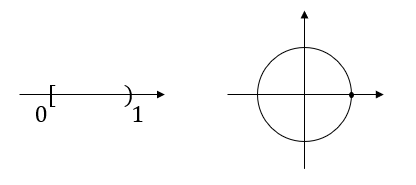
What homeomorphism really means is that the two spaces before and after the map should have the same topological properties. In the example above, the two topological spaces have completely different properties: the latter can be covered finitely, while the former cannot.

Finite cover theorem: every open cover of a finite closed interval $[a,b]$ has a finite subcover.

On $R$, this theorem is an expression of the continuity of the real numbers. For $(a,b)$, there are infinitely many $\epsilon$-neighborhoods near $a$ and $b$. Either you include the two endpoints $a,b$ directly, forming a closed interval and getting a finite cover, or if you do not want to include the endpoints, you must use infinitely many sets to approach them, that is, infinitely many open sets to cover $(a,b)$.

Going one step further, a diffeomorphism is a smooth homeomorphism. Locally, the two spaces before and after the map can be approximated linearly and treated as the same. The feeling behind diffeomorphism is that points that were not too far apart originally are still not too far apart after the map.

Examples

1. Stereographic projection: Let the upper sphere be $S^2=\lbrace(x,y,z) \vert x^2+y^2+z^2=1,z>0 \rbrace$, and take the north pole $N$ to be $(0,0,1)$. As in the figure, define the stereographic map $h: S^2 \backslash N \rightarrow R^2$, sending the coordinate $(x,y,z)$ to the plane coordinate $(u,v,0)$.

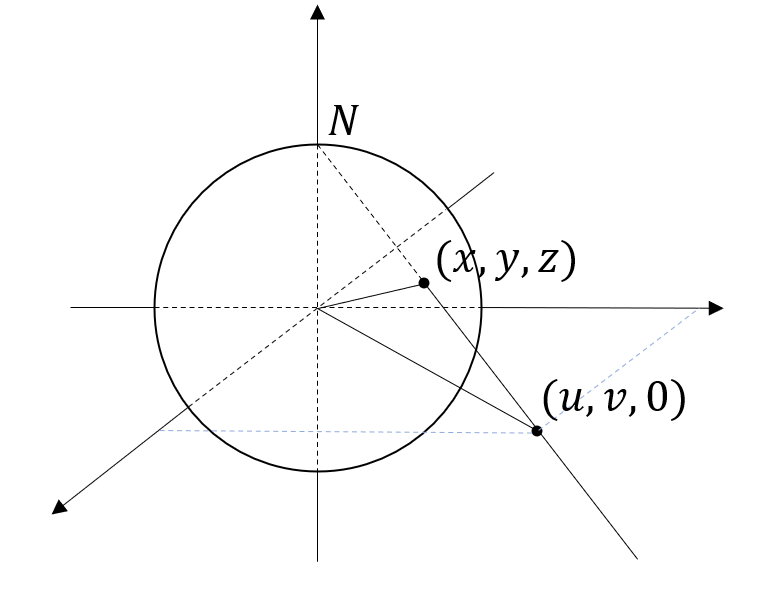
Give the sphere $S^2$ the subspace topology inherited from three-dimensional Euclidean space, and give the target plane the usual Euclidean topology. Clearly $h$ is a bijection. Proving that $h$ is continuous means showing that both $h$ and $h^{-1}$ are continuous.

To verify that $h$ is continuous, it is enough to check that the preimage of each basic open set is open. In other words, take the preimage of a small open disk around $(u,v,0)$ in the plane and check that it is open. The argument for $h^{-1}$ is the same.

We can also solve explicitly for $h$, in which case continuity becomes very natural.

2. Peano curve: Suppose $\Delta$ is an equilateral triangle with side length $1/2$. Construct a sequence of continuous maps $f\_n:[0,1] \rightarrow \Delta$ as follows:

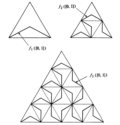
At each step, every triangle is divided into four smaller equilateral triangles. On the plane $R^2$, take the usual Euclidean topology. Given two points $x$ and $y$, define their distance as $\vert \vert x - y \vert \vert$.

Suppose $n \geq m$. For $t \in [0,1]$, we can always find a triangle with side length less than $1/2^m$ that contains both $f\_m(t)$ and $f\_n(t)$. So $\vert \vert f\_m(t)-f\_n(t) \vert \vert \leq 1/2^m$ holds for every $t \in [0,1]$. That is, the sequence of functions $f\_n$ converges uniformly, and its limit function is $f$. Since each function is continuous, $f$ is also continuous.

Now take a point $x$ inside the triangle and a neighborhood $U$ of $x$ in $R^2$. Choose $U$ large enough so that the disk centered at $x$ with radius $1/2^{N-1}$ is contained in $U$, and choose $t\_0 \in [0,1]$ such that:

Since for every $t \in [0,1]$ we have

by the triangle inequality,

So $f(t\_0)$ must lie in $U$. In other words, every point inside the triangle is a limit point of the set $f([0,1])$. Since the domain is closed, the image of a continuous map is also closed, so it must contain all of its limit points. Therefore the image of the map is the entire triangle.

Compactness

Where compactness comes from: In analysis, continuous functions on closed intervals have very good properties. For example, they are bounded, and they attain maximum and minimum values. We want to generalize these properties. In the proofs, the finite subcover property appears again and again. The finite cover property of a set is exactly the mechanism behind why closed intervals behave so well, and this mechanism is called the “compactness property” (Compactness) of a set.

Open cover: Let $X$ be a topological space. For a family of open subsets $\lbrace U\_i\rbrace$ of $X$, we call $\lbrace U\_i\rbrace$ an open cover of $X$ if $\cup{U\_i}=X$. If we can choose finitely many open sets $\lbrace U\_j\rbrace$ from $\lbrace U\_i\rbrace$ such that $\cup{U\_j}=X$, then $\lbrace U\_j\rbrace$ is a finite subcover of the original open cover $\lbrace U\_i\rbrace$ of $X$.

Compactness: Let $X$ be a topological space. If every open cover of $X$ has a finite subcover, then $X$ is compact, and we call it a compact space. Let $Y$ be a subset of $X$. We say $Y$ is a compact subset of $X$ if $Y$ is compact under the subspace topology.

One important role of compactness is that it turns infinity into finiteness. For example, it proves the classical result in analysis known as the extreme value theorem: a continuous function on a closed interval attains its maximum and minimum.

Since $f$ is continuous, $f$ is locally bounded. Take any $x \in [a,b]$. There exists a neighborhood $U\_x$ of $x$ such that $f$ has maximum and minimum values on $U\_x$. As $x$ ranges over $[a,b]$, all the $\lbrace U\_x \rbrace$ form an open cover of $[a,b]$. Since $[a,b]$ is compact, we can choose a finite subcover from $\lbrace U\_x \rbrace$. Since there are only finitely many of them, we can choose the largest and smallest among their local extrema. This is why a continuous function on a closed interval attains its maximum and minimum.

Of course, this approach takes finite covers as an assumption. Without using that condition, we would prove it using nested closed intervals.

Another important role of compactness is that it lets us integrate without worrying too much. For example, if $f:[a,b] \rightarrow R$ is continuous, then $\int\_{a}^{b}f(x)dx$ is fine. If we replace the domain by $[a,b)$, then improper integrals appear, and convergence becomes an issue. In topology, many topological invariants are defined through integration, so compactness is very important.

Compactness of product spaces: If the topological spaces $X$ and $Y$ are compact, then $X \times Y$ is a product space. Define the family of subsets of $X \times Y$ by $\mathscr{F} = \lbrace U \times Y \vert U \subset X, V \subset Y \rbrace$, where both $U$ and $V$ are open sets. Then $\mathscr{F}$ generates a product topology on $X \times Y$, and under this topology, $X \times Y$ is also compact.

The proof is easy, but first we need to explain that $\mathscr{F}$ really does generate a topology on $X \times Y$ (that is, $\mathscr{F}$ is a basis). This means proving that the union of all sets in $\mathscr{F}$ is the whole space, and that $\mathscr{F}$ is closed under finite intersections. Both of these conditions are actually obvious.

Remark

The relationship between compact sets and closed sets: compact does not imply closed. For example, use the universal counterexample: $X=\lbrace 0, 1 \rbrace$ with topology $\mathscr{F} = \lbrace \lbrace 0 \rbrace, \lbrace 0,1 \rbrace , \varnothing\rbrace$. Finite covers are automatic in this topology, so every set is compact. But the set ${0}$ is not closed. If it were closed, then its complement ${1}$ would have to be open, which is clearly a contradiction. In algebraic geometry, there is also a large class of sets (affine open subsets) that are compact but not closed.

If the topological space is Hausdorff, then compact sets are closed.

Let $X$ be a Hausdorff space, and let $Y$ be a subset of $X$ that is compact. We want to prove that $X \backslash Y$ is open. Take a point $x\_0$ in $X \backslash Y$. For every point $y$ in $Y$, by the Hausdorff condition, there are two corresponding open sets $U\_y$ and $V\_y$ such that $x \in U\_y, y \in V\_y$ and $U\_y \cap V\_y = \varnothing$. As $y$ ranges over all of $Y$, we get an open cover $\lbrace V\_y \rbrace$ of $Y$. Therefore there is a finite subcover $\lbrace V\_{y\_i} \rbrace$. Correspondingly, we get a finite family of open sets $\lbrace U\_{y\_i} \rbrace$ containing $x\_0$. Intersect all the $\lbrace U\_{y\_i} \rbrace$. Since this is a finite intersection of open sets, it is open, and it is strictly contained in $X \backslash Y$. Now let $x\_0$ range over all of $X \backslash Y$. Then $X \backslash Y$ is open, so $Y$ is closed.

So compact subsets of $R^n$ are always closed and bounded, because $R^n$ is a metric space, and metric spaces are Hausdorff. Boundedness can be obtained from finite covers. The converse is also true.

The relationship between compactness and continuous maps: Under a continuous map, the image of a compact set is compact. From this we can further conclude: a continuous real-valued function on a compact space is bounded and attains its maximum and minimum.

Take an open cover of the image set (we do not yet know whether it has a finite subcover). The preimage of each open set is open, so pulling back gives an open cover of the original space. Since the original space is compact, this pulled-back cover has a finite subcover. The pullback process preserves the indexing, so the same indices give a subcover of the image cover. Therefore the open cover of the image also has a finite subcover, and the image is compact.

Other Forms of Compactness

Limit point compactness (limit point compact): Let $X$ be a topological space. We say $X$ is limit point compact if every infinite subset of $X$ has a limit point.

• Compact $\Rightarrow$ limit point compact.

Suppose $X$ is compact. Take any $A \subset X$ where $A$ is infinite. Suppose $A$ has no limit point. Then for every $x \in X$, there exists an open set $U\_x$ in $X$ such that $(U\_x \backslash {x}) \cap A=\varnothing$. In other words, $U\_x=\lbrace x\rbrace$ or $U\_x$ is empty. Then as $x$ ranges over $X$, the union of all $U\_x$ is $X$, that is, $\cup U\_x = X$. Since $X$ is compact, we can choose finitely many $U\_x$ from $\lbrace U\_x \rbrace$ whose union covers $X$. But each $U\_x$ is at most a singleton, so this is a contradiction.

• Limit point compact $\nRightarrow$ compact.

Counterexample: $\mathbb{Z}\_{+} \times Y$, where $\mathbb{Z}\_{+}=\lbrace 1, 2, 3,... \rbrace$ has the discrete topology, and $Y=\lbrace 0, 1 \rbrace$ has the trivial topology. The product space $\mathbb{Z}\_{+} \times Y$ is limit point compact, but not compact.

Sequential compactness (sequentially compact): Let $X$ be a topological space. We say $X$ is sequentially compact if every infinite sequence of points in $X$ has a convergent subsequence.

• Compact $\nRightarrow$ sequentially compact.

Counterexample: $[0,1]^{[0,1]}$ is an infinite product space. Since $[0,1]$ is compact, $[0,1]^{[0,1]}$ is also compact (a finite product of compact spaces is compact; Tychonoff’s theorem says that an infinite product of compact spaces is also compact). But it is not sequentially compact.

• Sequentially compact $\nRightarrow$ compact.

• Sequentially compact $\Rightarrow$ limit point compact.

• Limit point compact $\Rightarrow$ sequentially compact.

Counterexample: On $R$, do not take the usual topology. Instead take the right topology: $\mathscr{F}=\lbrace (a, +\infty ) \vert a \in R \rbrace$. Take $\lbrace x\_n\rbrace=-n,n \in \mathbb{N}$. Clearly it has no convergent subsequence (note that non-convergence here is proved in the right topology), so it is not sequentially compact.

But it is limit point compact. For every nonempty $A \subset R$, choose $x\_0 \in A$. Then $x\_0 - 1$ is a limit point of $A$, because for any open set $U \subset R$, if $x\_0-1 \in U$, then $U$ must be $(x, +\infty), x < x\_0$. Therefore $(U \backslash \lbrace x\_0 - 1 \rbrace) \cap A$ contains at least the point $x\_0$. So $x\_0 - 1$ must be a limit point of $A$, and the space is limit point compact.

• In metric spaces, limit point compactness, sequential compactness, and compactness are equivalent.

Categories

Example of vector spaces: Suppose $V$ and $W$ are two vector spaces over a field $K$. Construct $V \times W$ as a vector space over $K$, with addition and scalar multiplication defined as follows:

There are two natural linear maps (projection maps) on $V \times W$: $\pi\_1 : V \times W \rightarrow V$ and $\pi\_2 : V \times W \rightarrow W$. The vector space $V \times W$, together with these two linear maps $\pi\_1,\pi\_2$, has the following property:

For any vector space $Z$ and linear maps $f : Z \rightarrow V$ and $g : Z \rightarrow W$, there exists a unique linear map $h : Z \rightarrow V \times W$ such that the following diagram commutes.

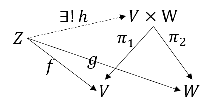
First, $h$ certainly exists: just define $h(v)=(f(v),g(v))$. It is easy to check that $h$ is a linear map, and that its compositions with $\pi\_1,\pi\_2$ match the diagram above. Next we prove uniqueness.

Suppose there is another linear map $h^{\prime}$ satisfying the commutative diagram condition, so $\pi\_1 \circ h^{\prime}=f$ and $\pi\_2 \circ h^{\prime}=g$. For every $v \in Z$, write $h^{\prime}(v)=(h^{\prime}\_1(v),h^{\prime}\_2(v))$. Then:

Therefore $h^{\prime}\_1(v)$ is exactly $f(v)$ and $h^{\prime}\_2(v)$ is exactly $g(v)$, so $h^{\prime}=h$.

Example of groups: Suppose $G$ and $H$ are two groups. Construct $G \times H$ as a product group. Define multiplication by:

It is easy to check that $G \times H$ is still a group. On this group, there are two natural group homomorphisms $\pi\_1 : G \times H \rightarrow G$ and $\pi\_2 : G \times H \rightarrow H$. The group $G \times H$, together with these two natural homomorphisms $\pi\_1,\pi\_2$, has the following property:

For any group $K$ and group homomorphisms $f : K \rightarrow G$ and $g : K \rightarrow H$, there exists a unique group homomorphism $h : K \rightarrow G \times H$ such that the following diagram commutes.

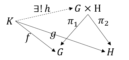
In fact, for any $k \in K$, just define $h(k)=(f(k),g(k))$. The rest of the proof is the same as above.

Example of topological spaces: Suppose $X$ and $Y$ are two topological spaces. Construct $X \times Y$ as a product topological space. There are two natural maps on the space, $\pi\_1 : X \times Y \rightarrow X$ and $\pi\_2 : X \times Y \rightarrow Y$. These maps $\pi\_1,\pi\_2$ are continuous (prove it by checking that preimages of open sets are open; this is easy). Then the topological space $X \times Y$, together with the two continuous maps $\pi\_1,\pi\_2$, has the following property:

For any topological space $Z$ and continuous maps $f : Z \rightarrow X$ and $g : Z \rightarrow Y$, there exists a unique continuous map $h : Z \rightarrow X \times Y$ such that the following diagram commutes.

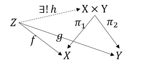
The existence and uniqueness of $h$ are the same as above. The continuity of $h$ needs a separate explanation.

Category: A category $C$ consists of the following four pieces of data:

1. Some things called objects, $Ob(C)$ (Object)
2. Some things called morphisms, $Hom(C)$ (Morphism)
3. A map $s:Hom(C) \rightarrow Ob(C)$ (the Source map), and a map $t:Hom(C) \rightarrow Ob(C)$ (the Target map). If for every $f \in Hom(C),s(f)=X,t(f)=Y$, we also write $f: X \rightarrow Y$. In addition, write $Hom\_C(X,Y)=\lbrace f \in Hom(C) \vert s(f)=X,t(f)=Y \rbrace$ for the collection of all morphisms from $X$ to $Y$ in the category $C$.
4. An operation $\circ : Hom(X,Y) \times Hom(Y,Z) \rightarrow Hom(X,Z)$, called composition (Composition).

These four pieces of data satisfy:

1. Associativity: for every $X,Y,Z,W$, if there are morphisms $f:X \rightarrow Y, g: Y \rightarrow Z,h:Z \rightarrow W$, then $(h \circ g) \circ f=h \circ (g \circ f)$.
2. Identity morphisms: for every $x \in Ob(C),\exists 1\_x:X \rightarrow X$ such that for every $f:X \rightarrow Y,g: Z \rightarrow X$, we have $f \circ 1\_x = f, 1\_x \circ g=g$. (The identity morphism is unique.)

Isomorphism: Let $C$ be a category, and let $X,Y$ be two objects in $C$. We say $X$ and $Y$ are isomorphic if there exist two morphisms $f:X \rightarrow Y,g: Y \rightarrow X$ such that $f \circ g=1\_Y,g \circ f = 1\_X$.

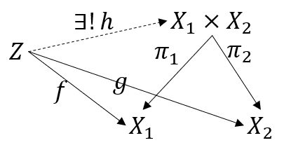
Product in a category: Let $C$ be a category, and let $X\_1,X\_2$ be two objects in $C$. The product of $X\_1,X\_2$ consists of the following data:

1. $Y \in Ob(C)$, written $Y:=X\_1 \times X\_2$.
2. Morphisms $\pi\_1:Y \rightarrow X\_1,\pi\_2: Y \rightarrow X\_2$.

It satisfies the following universal property: for every $Z \in Ob(C)$ and two morphisms $f: Z \rightarrow X\_1,g : Z \rightarrow X\_2$, there exists a unique morphism $h: Z \rightarrow Y$ such that the following diagram commutes.

Property: if the product of $X\_1$ and $X\_2$ exists, then it is unique up to isomorphism.

Suppose that besides $Y$, there is also $Y^{\prime}=X\_1 \times X\_2$. By the universal property above, set $Z$ to be $Y^{\prime}$. Then by the uniqueness of identity morphisms, we know $Y^{\prime}=Y$.

Connectedness

Let $X$ be a topological space. We say $X$ is connected if: whenever $U$ and $V$ are open sets with $U \cap V=\varnothing$ and $X=U \cup V$, at least one of $U$ and $V$ is empty.

An equivalent characterization: a topological space $X$ is connected if and only if the only subsets of $X$ that are both open and closed are the empty set and the whole space.

Important example: $R$ is connected.

Suppose $R$ is not connected. Then there exists an open set $U \subset R$ such that $U$ is both open and closed, and $U$ is neither empty nor the whole space. Since $U$ is not the whole space, there exists at least one $x\_1 \in R \backslash U$; since $U$ is not empty, there exists at least one $x\_2 \in U$. Without loss of generality, assume $x\_1 < x\_2$. Consider $S=\lbrace x \in R | x \geq x\_1,[x1,x] \subset R \backslash U \rbrace$. Clearly $S$ is nonempty and bounded above, with $x\_2$ as an upper bound. By the axioms of the real numbers, $S$ has a supremum $s=sup S$. Now split into two cases: First, if $s$ lies in $U$, so $s \in U$, then since $U$ is open, there exists $\delta > 0$ such that $(s-\delta , s + \delta) \subset U$. Pick any number, say $s-\delta / 2 \in U$. It is also an upper bound of $S$, but $s$ is the least upper bound. This gives an upper bound smaller than the least upper bound, a contradiction. Second, if $s \notin U$, then since $U$ is closed, $R \backslash U$ is open. So there exists $\delta > 0$ such that $(s-\delta , s + \delta) \subset R \backslash U$. Using the same trick as above also gives a contradiction. Therefore, $R$ is connected.

Checking connectedness of every space or set directly from the definition is painful, so we need the following important result.

The image of a connected space under a continuous map is still connected. (That is, connectedness is a topological invariant.)

Take a nonempty subset of the image that is both open and closed. Since the map is continuous, its preimage must also be both open and closed. And the map is surjective ($X \rightarrow Y$ may not be surjective, but then we can consider $X \rightarrow f(X)$ with the subspace topology; $f$ is still continuous and is surjective onto the subspace). So the preimage must be the whole space.

For example, the space $S^1$ is connected.

We can use the map $f(x)=exp(i2\pi x)$. Since $R$ is connected and the map is continuous, we know $S^1$ is connected.

For example, $S^1$ and $R$ are not homeomorphic.

First proof: use compactness as a topological invariant. $S^1$ is compact, but $R$ is not compact, so they definitely cannot be homeomorphic.

Second proof: use connectedness as a topological invariant. Suppose $S^1$ and $R$ are homeomorphic, with the map realized by $\phi$. Take a point $p$. Then under $\phi: S^1 \backslash \lbrace p\rbrace \rightarrow R \backslash \lbrace \phi(p) \rbrace$, connectedness remains a topological invariant. The unit circle with this point removed is still connected (by stereographic projection), but $R \backslash \lbrace \phi(p) \rbrace$ is clearly disconnected, a contradiction.

Proposition: Let $X$ be a topological space, and let $\lbrace F\_{a} \rbrace\_{a \in I}$ be a family of connected subsets of $X$ such that every pair intersects nontrivially, and $X = \cup\_{a \in I}F\_a$. Then $X$ is connected.

For example, $S^1$ and $S^2$ are not homeomorphic.

If we remove two points from $S^1$, it becomes disconnected, but if we remove two points from $S^2$, it is still connected. Now let us explain why $S^2$ with two points removed is still connected.

Since $S^2 \backslash \lbrace p \rbrace$ is homeomorphic to $R^2$, proving that $S^2 \backslash \lbrace p\_1,p\_2 \rbrace$ is connected is equivalent to proving that $R^2 \backslash \lbrace p \rbrace$ is connected. And $R^2 \backslash \lbrace p \rbrace$ is homeomorphic to $R^2 \backslash \lbrace(0,0) \rbrace$. So after removing the origin, we can build a nested family of connected annular regions centered at the origin whose union is the whole space $R^2 \backslash \lbrace(0,0) \rbrace$. This shows that $R^2 \backslash \lbrace(0,0) \rbrace$ is connected.