Theory of Curves
A Few Results I Often Forget
- Double cross product formula
- Lagrange identity
- Suppose the vector-valued function ${a}(t)$ is nowhere zero and continuously differentiable. Then the length of ${a}(t)$ is constant if and only if:
Regular Parametric Curves
A parametric curve ${\textbf{r} }(t)$ is a regular parametric curve if it satisfies the following conditions:
- ${\textbf{r} }(t)$ is at least a vector-valued function of the variable $t$ with continuous derivatives up to order three.
- Every point on the curve is a regular point; that is, for any $t$, ${\textbf{r} }^{\prime}(t) \neq 0$.
The direction in which the parameter increases is called the positive direction of the parametric curve.
For a regular parametric curve, arc length is an invariant of the curve:
Basically, we can think of ${\textbf{r} }^{\prime}(t)$ as velocity, and arc length is the distance obtained by integrating speed.
Also, the arc length $s$ can be used as a parameter of the curve. If $\vert {\textbf{r} }^{\prime}(t) \vert \equiv 1$, it is called an arc-length parameter.
Why arc length can be used as a curve parameter:
First we have:
So $s(t)$ is monotonically increasing with respect to $t$. Therefore $s(t)$ has an inverse function $t=t(s)$, and hence $s$ can be used as a parameter instead of $t$.
If the curve is parameterized by arc length, that means the tangent vector field of the curve is a unit vector field. (Think of ${\textbf{r} }^{\prime}(t)$ as velocity: using an arc-length parameter means the motion has constant speed 1.)
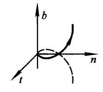
Frenet Frame
Take a regular parametric curve ${\textbf{r} }(s)$, with $s$ chosen as the arc-length parameter. To build the frame:
- Tangent vector
Differentiate ${\textbf{r} }(t)$ directly with respect to $t$ to get the tangent vector:
- Principal normal vector
Since $s$ is the arc-length parameter, $\vert {\textbf{t} }(s) \vert = 1$, namely $<{\textbf{t} }(s), {\textbf{t} }(s)>=1$. Differentiating this gives $<{\textbf{t} }^{\prime}(s), {\textbf{t} }(s)>=0$. So we have found a normal vector ${\textbf{t} }^{\prime}(s)$. Although $\vert {\textbf{t} }(s) \vert = 1$, $\vert {\textbf{t} }^{\prime}(s) \vert$ is not necessarily unit length. To make ${\textbf{n} }$ a unit vector, define the curvature:
Then redefine the unit normal vector we found as:
- Binormal vector
${\textbf{t} }$ and ${\textbf{n} }$ are perpendicular, so define the binormal vector directly by the cross product:
Differentiate the binormal vector once more:
That is, $d{\textbf{b} } / ds$ is perpendicular to the tangent vector ${\textbf{t} }$, so $d{\textbf{b} } / ds$ must be parallel to ${\textbf{n} }$. Thus set:
Multiply both sides by ${\textbf{n} }$. Since it is a unit vector, we get:
This is called the torsion of the curve. It measures how much the curve deviates from being planar.
In summary, the Frenet frame of a curve is $\lbrace {\textbf{r} }; {\textbf{t} },{\textbf{n} },{\textbf{b} }\rbrace$.
Frame Equations of Motion
This just means differentiating the Frenet frame. Since the frame itself is an orthonormal basis, after differentiation it can still be expressed linearly in terms of the frame itself. The result is:
The first row follows directly from the definition. The third row also follows directly from the definition of torsion above.
For the second row, differentiate both sides of ${\textbf{n} }={\textbf{b} } \times {\textbf{t} }$.
Fundamental Theorem of Curve Theory
That is: up to rigid motions, curvature and torsion uniquely determine a curve (for a regular arc-length parameterized curve, with curvature nowhere zero).
The essence of the proof is to show that the frame equations of motion have a unique solution, and that the solution is indeed a regular curve parameterized by arc length.
The Two Fundamental Forms of a Surface
A surface is usually written as $\textbf{r}=\textbf{r}({u^1},{u^2})$ or $\textbf{r}=\textbf{r}(u,v)$. To make the later Einstein summation notation convenient, I will use the first notation directly. Also, partial derivatives are denoted by $\textbf{r}\_{u^i}$, or more simply by $\textbf{r}\_i$.
Regular parametric surface:
- The continuous map $S \rightarrow R^3$ is a homeomorphism.
- It is smooth and differentiable at least three times.
- Regularity: the map is injective; equivalently, the Jacobi matrix has full rank; equivalently, $\textbf{r}\_{u^1}$ and $\textbf{r}\_{u^2}$ are linearly independent.
Why require a homeomorphism: a one-to-one map alone is not enough. Two points that are very close in $R^2$ might be mapped very far apart in $R^3$. So we want the differential structure to be controlled as well, and that is why we require a homeomorphism.
The definition of a surface above is local. The full definition of a surface is obtained by gluing together locally defined surface patches. For planes and cylinders, the local definition can be equivalent to a global one, but for spheres and similar surfaces it cannot. Spheres, tori, and so on are bounded closed subsets of $R^3$, hence compact sets, so we cannot find an open set homeomorphic to the whole surface.
For a regular parametric surface, $\textbf{r}\_u$ and $\textbf{r}\_v$ are two tangent vectors. They are linearly independent, and the space they span is the tangent space, $T\_pS\lbrace \textbf{r}\_{u^1},\textbf{r}\_{u^2}\rbrace$. The cross product of the two tangent vectors gives a normal vector (which needs to be normalized), $\textbf{n}= \textbf{r}\_{u^1} \times \textbf{r}\_{u^2} / \vert \textbf{r}\_{u^1} \times \textbf{r}\_{u^2} \vert$. Therefore the two tangent vectors together with the normal vector form the natural frame of the surface, $\lbrace \textbf{r}\_{u^1}, \textbf{r}\_{u^2}, \textbf{n} \rbrace$.
For $\textbf{r}=\textbf{r}({u^1},{u^2})$, take the first differential:
Then the first fundamental form is the square of the length of the tangent vector $d{\textbf{r} }$:
Here $g\_{ij}$ denotes the coefficient matrix of the first fundamental form. The second fundamental form is:
Here $h\_{ij}$ denotes the coefficient matrix of the second fundamental form. The equality between corresponding entries of the two matrices above uses:
Just take partial derivatives on both sides of these two equations.
The First Fundamental Form Describes Metric Properties
The area element at a point of the surface is:
The first fundamental form is always positive definite.
The Second Fundamental Form Describes Bending Properties
Using the usual $(u,v)$ notation for $(u^1,u^2)$, take a small displacement on the surface $S$ from the point $(u\_0,v\_0)$ to $(u\_0+\Delta u,v\_0+\Delta v)$. We look at how much this displacement differs in the normal direction at the initial point of the normal line, namely:
Take the limit of the expression above. The first expanded term lies in the tangent plane, so its inner product with the normal is directly 0. The third term is a higher-order infinitesimal and vanishes in the limit. What remains is the inner product of the second term with the normal, which is exactly the second fundamental form.
The second fundamental form may be positive definite or negative definite; it may also be indefinite or degenerate.
Equations of Motion and Structure Equations of Surfaces
Equations of Motion
With the natural frame $\lbrace \textbf{r}\_{u^1}, \textbf{r}\_{u^2}, \textbf{n} \rbrace$ in hand, we can now derive the equations of motion for a surface. We have:
Now compute $\Gamma,\Lambda,\Theta,\Delta$ one by one:
For the second equation, since $\textbf{n}$ is a unit normal vector, the derivative of the unit normal vector is a vector in the tangent plane and has no normal component. That is:
Therefore:
For the second equation, take the inner product of both sides with $\textbf{r}\_k$:
That is:
So:
Here $g^{ik}$ is the inverse matrix of $g\_{ik}$. It is just a notation. We have $g^{ik}g\_{ik}=\delta\_i^k$.
For convenience later, write:
Then the second equation finally becomes (here I pull out the minus sign, which makes later manipulations cleaner):
Now look at the first equation. Take the inner product of both sides with $\textbf{n}$:
Therefore:
The only thing left is $\Gamma$. Take the inner product of both sides with $\textbf{r}\_m$:
To compute $\langle\textbf{r}\_{ij}, \textbf{r}\_m\rangle$, consider:
Cycling the indices gives two more equations:
Add the first two equations and subtract the third, and we can solve for $\langle\textbf{r}\_{ij}, \textbf{r}\_m\rangle$:
So we have:
Finally, the equations of motion for a surface are:
where:
Structure Equations
Next, derive the structure equations of a surface. The idea is the commutativity of second and third partial derivatives. Differentiate the first equation of motion once more:
Swap the order of differentiation in the last two indices:
The two expressions should be equal, so the corresponding tangential and normal parts must be equal respectively:
The first equation, from the tangential part, is called the Gauss equation. The second equation, from the normal part, is called the Codazzi equation. These two equations are necessary conditions for forming a parametric surface.
Similarly, we can perform the same operation on the second equation of motion, but it still gives the Codazzi equation and no new equation appears.
Number of Independent Equations in the Structure Equations
Normal Curvature
This comes from studying the curvature vector of a curve on a surface. Let the curve be ${\textbf{r} }(s)={\textbf{r} }({u^1}(s),{u^2}(s))$, where $s$ is the arc-length parameter. Then the unit tangent vector on the curve is:
Differentiate once more to get the curvature vector:
This vector (the normal vector of the curve) can be decomposed into two parts: a tangential part and a normal part relative to the surface. The normal part is the normal curvature, measuring the bending of the surface relative to $R^3$; the tangential part is the geodesic curvature, measuring how the curve bends relative to the surface.
So we examine the normal direction. Take the dot product of the expression above with the surface normal vector ${\textbf{n} }$:
The defined $\kappa\_n$ is the normal curvature of the surface at this point along the chosen unit tangent vector. We can see that:
- The value of the normal curvature depends on the selected point.
- The normal curvature depends only on the second fundamental form.
- The normal curvature depends on the tangent vector at the point under consideration (because we study it through curves on the surface), but it does not depend on the particular curve. If two different curves have the same tangent vector at this point, then their normal curvature is the same.
Note that the derivation of normal curvature is based on a unit tangent vector at a point:
Given a unit tangent vector ${v}=\lambda\_1 {\textbf{r}\_1} + \lambda\_2 {\textbf{r}\_2}$, the pair $\lbrace \lambda\_1, \lambda\_2 \rbrace$ corresponds to $\lbrace du^1/ds, du^2/ds\rbrace$. So the normal curvature is also:
where $h\_{ij}$ is the coefficient matrix of the second fundamental form.
Next, change the form a bit so that normal curvature becomes a function of the “direction” at a point on the surface.
So the whole expression is a function of $du/dv$, that is, a function of the “direction.” Normal curvature is the degree of bending at a point of a surface along a specified direction. Therefore, naturally, the directions where normal curvature reaches its maximum and minimum values are the principal directions of the surface at that point, and the corresponding normal curvatures are the principal curvatures of the surface at that point.
Following the theory of curves, differential geometry needs to analyze the motion of frames. On a surface, this is the frame $\lbrace {\textbf{r}\_{u^1} }, {\textbf{r}\_{u^2} }, {\textbf{n} } \rbrace$. We have:
These are the frame equations of motion.
Why the second equation has no normal component:
Because $n$ is a unit normal vector, and the derivative of a unit normal vector is a vector in the tangent plane, so there is no normal component. That is:
Why there is a minus sign in front of the second equation: To make later conclusions look a bit nicer.
The $h\_{ij}$ in the first equation can be obtained by dotting both sides with the normal vector. That is:
In other words, $h\_{ij}$ is the coefficient of the second fundamental form.
Weingarten Map
For the second equation of motion above, the goal is to solve for $a\_i^j$. First write the equation in matrix form:
To bring together the two fundamental forms, multiply both sides on the left by $[\textbf{r}\_1, \textbf{r}\_2]$:
Here $h$ is the second fundamental form matrix, and $g$ is the first fundamental form matrix. We get:
Define a linear map $W$ from $T\_pS$ to $T\_pS$ by sending the basis vectors to:
The matrix of this map under the basis $\lbrace {\textbf{r}\_{u^1} }, {\textbf{r}\_{u^2} }\rbrace$ is exactly the matrix $A$ above. This linear map is called the Weingarten map on $TpS$, denoted by $W$.
Now take a unit tangent vector ${v}=\lambda\_1 {\textbf{r}\_{u^1} } + \lambda\_2 {\textbf{r}\_{u^2} }$ at a point on the surface. Its normal curvature (at that point) was given above:
Some Properties of the Weingarten Map
It is a self-adjoint transformation: $W({a}) \cdot {b} = {a} \cdot W({b})$. (The eigenvalues of a self-adjoint transformation are real.)
The eigenvalues and eigenvectors of the Weingarten map are precisely the principal curvatures of the surface at this point and their corresponding direction vectors.
Computing Principal Directions and Principal Curvatures
- Start with a local parameterization ${\textbf{r} }={\textbf{r} }({u^1},{u^2})$, and compute the normal vector ${\textbf{n} }$.
- Compute the matrices $g\_{ij}$ and $h\_{ij}$ of the two fundamental forms. For a two-dimensional surface, these correspond to the six parameters $EFGLMN$.
- Compute the Weingarten map matrix:
- Compute the determinant of $W$:
- Mean curvature: